Tidying Multi-Header Excel Data with R
Problem
If you’re lucky enough to work with a lot of data that arrives in the form of excel tables, you will most likely be familiar with data in the format below.
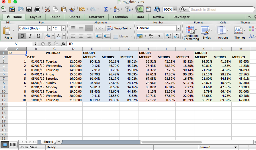
This format makes it easier for a human eye to read the data, but seriously hinders a computers ability to analyse it. So, if you prefer analysing and visualising your data with a programming language rather than staring at it in Excel we’re going to need to knock it into a tidier form before we can let the powers of R loose on it.
That means one column for each variable and one row for each observation of said variables. For this sample data set I would define that as columns for:
IDDATEWEEKDAYTIMEGROUPMETRIC1METRIC2METRIC3
Currently we have the metrics for each group spread out over 3 chunks with the group indicated by a top header (only in the first column of that group) and the metric headers below. Adding fuel to the fire, in the first chunk of columns you’ll notice the ID and WEEKDAY columns are floating up in row one with the others down in row 2 - nice.
Solution
A data frame in R can only take one set of column names that must be unique from each other so we need a method of reducing these headers into a single row of unique names by merging the group and metric information together with a separator. So group 1’s metric columns will be named GROUP1_METRIC1 GROUP1_METRIC2 GROUP1_METRIC3 and so forth for each group.
So let’s give it a go. These are the packages required:
library(tidyverse)
library(readxl)
library(hms) # to convert datetimes to hms class
library(zoo) # for the super useful na.locf0 function
If we read all of the data with read_excel what do we get?
path <- "../../static/my_data.xlsx"
raw_data <- read_excel(path)
raw_data
## # A tibble: 11 x 13
## ID X__1 WEEKDAY X__2 GROUP1 X__3 X__4 GROUP2 X__5 X__6 GROUP3
## <dbl> <chr> <chr> <chr> <chr> <chr> <chr> <chr> <chr> <chr> <chr>
## 1 NA DATE <NA> TIME METRI… METR… METR… METRI… METR… METR… METRI…
## 2 1.00 43466 Tuesday 0.5 0.467… 0.80… 0.30… 0.475… 5.98… 0.78… 0.843…
## 3 2.00 43467 Wednesd… 0.54… 0.822… 0.51… 0.27… 1.791… 0.80… 0.21… 0.469…
## 4 3.00 43468 Thursday 0.58… 0.891… 0.63… 0.51… 0.794… 0.74… 0.35… 0.281…
## 5 4.00 43469 Friday 0.625 0.247… 0.13… 0.93… 0.951… 0.35… 0.86… 0.480…
## 6 5.00 43470 Saturday 0.66… 0.286… 0.35… 0.47… 0.364… 6.03… 7.35… 6.769…
## 7 6.00 43471 Sunday 0.70… 0.416… 0.98… 0.64… 0.667… 0.48… 0.76… 0.927…
## 8 7.00 43472 Monday 0.75 0.401… 0.58… 5.40… 0.608… 0.89… 0.39… 9.688…
## 9 8.00 43473 Tuesday 0.79… 0.643… 0.87… 0.67… 0.602… 0.77… 0.52… 0.659…
## 10 9.00 43474 Wednesd… 0.83… 0.657… 0.39… 0.37… 0.870… 0.30… 0.51… 0.898…
## 11 10.0 43475 Thursday 0.875 0.749… 0.47… 0.88… 0.820… 0.10… 2.90… 0.423…
## # ... with 2 more variables: X__7 <chr>, X__8 <chr>a mess.
The first row has been set as the column names with blank names assigned as X__* by readxl. Also every column has a character class because the second row headers have been considered as data.
Building our own column names with code
So before attempting to actually read in the data lets try to form the single set of column names we need. To do this, I’m going to first get the headers in row 1 as a character vector and replace the missing column name pattern X__* with an NA.
Like so:
head1 <- read_excel(path, col_names = TRUE) %>%
  names() %>%
  str_replace("X__\\d*", NA_character_)

head1
## [1] "ID" NA "WEEKDAY" NA "GROUP1" NA NA
## [8] "GROUP2" NA NA "GROUP3" NA NATo do the same for the headers in row 2 we do the same thing but add a skip = 1 argument to read_excel which tells it to ignore the first row entirely.
head2 <- read_excel(path, skip = 1, col_names = TRUE) %>%
  names() %>%
  str_replace("X__\\d*", NA_character_)

head2
## [1] NA "DATE" NA "TIME" "METRIC1"
## [6] "METRIC2" "METRIC3" "METRIC1__1" "METRIC2__1" "METRIC3__1"
## [11] "METRIC1__2" "METRIC2__2" "METRIC3__2"Because we had non-unique column names in this case read_excel has assigned some __* patterns to the metric names which we also want to get rid of.
head2 <- head2 %>% str_remove("__\\d*")
head2
## [1] NA "DATE" NA "TIME" "METRIC1" "METRIC2" "METRIC3"
## [8] "METRIC1" "METRIC2" "METRIC3" "METRIC1" "METRIC2" "METRIC3"To deal with the rogue ID and WEEKDAY columns that were in row 1 with nothing below in row 2, we want to move them from head1 into head2 then replace with NA in head1
ncols <- length(head1)

for (n in 1:ncols) {
  if (is.na(head2[n])) {
    head2[n] <- head1[n]
    head1[n] <- NA_character_
  }
}

head1
## [1] NA NA NA NA "GROUP1" NA NA
## [8] "GROUP2" NA NA "GROUP3" NA NAhead2## [1] "ID" "DATE" "WEEKDAY" "TIME" "METRIC1" "METRIC2" "METRIC3"
## [8] "METRIC1" "METRIC2" "METRIC3" "METRIC1" "METRIC2" "METRIC3"Getting there! Next we need to fill out each group name so that it occurs 3 times to match each metric, rather than just once. To do this we can convert the vector to a 1 column tibble or data frame then use the zoo::na.locf0() that replaces NAs with nearest non-NA above it, then pull it back into a vector.
head1 <- tibble(head1) %>%
  mutate(head1 = zoo::na.locf0(head1)) %>%
  pull()

head1
## [1] NA NA NA NA "GROUP1" "GROUP1" "GROUP1"
## [8] "GROUP2" "GROUP2" "GROUP2" "GROUP3" "GROUP3" "GROUP3"We’re finally at the stage where we can combine the headers. Using map_chr we can ask R to merge headers with a _ separator only if there is a non-NA in head1 and head2, otherwise we only need the head2 name.
headers <- map_chr(1:ncols, ~ {
  case_when(
    !is.na(head1[.x]) & !is.na(head2[.x]) ~ paste(head1[.x], head2[.x], sep = "_"),
    TRUE ~ head2[.x]
  )
})

headers
## [1] "ID" "DATE" "WEEKDAY" "TIME"
## [5] "GROUP1_METRIC1" "GROUP1_METRIC2" "GROUP1_METRIC3" "GROUP2_METRIC1"
## [9] "GROUP2_METRIC2" "GROUP2_METRIC3" "GROUP3_METRIC1" "GROUP3_METRIC2"
## [13] "GROUP3_METRIC3"🙌
Import the data with new headers
Now we can read in the data, ignore both header rows and supply our own column names to read_excel
raw_data <- read_excel(path, skip = 2, col_names = headers)

raw_data
## # A tibble: 10 x 13
## ID DATE WEEKDAY TIME GROUP1_METRIC1
## <dbl> <dttm> <chr> <dttm> <dbl>
## 1 1.00 2019-01-01 00:00:00 Tuesday 1899-12-31 12:00:00 0.468
## 2 2.00 2019-01-02 00:00:00 Wednesday 1899-12-31 13:00:00 0.822
## 3 3.00 2019-01-03 00:00:00 Thursday 1899-12-31 14:00:00 0.891
## 4 4.00 2019-01-04 00:00:00 Friday 1899-12-31 15:00:00 0.248
## 5 5.00 2019-01-05 00:00:00 Saturday 1899-12-31 16:00:00 0.286
## 6 6.00 2019-01-06 00:00:00 Sunday 1899-12-31 17:00:00 0.416
## 7 7.00 2019-01-07 00:00:00 Monday 1899-12-31 18:00:00 0.402
## 8 8.00 2019-01-08 00:00:00 Tuesday 1899-12-31 19:00:00 0.643
## 9 9.00 2019-01-09 00:00:00 Wednesday 1899-12-31 20:00:00 0.657
## 10 10.0 2019-01-10 00:00:00 Thursday 1899-12-31 21:00:00 0.750
## # ... with 8 more variables: GROUP1_METRIC2 <dbl>, GROUP1_METRIC3 <dbl>,
## # GROUP2_METRIC1 <dbl>, GROUP2_METRIC2 <dbl>, GROUP2_METRIC3 <dbl>,
## # GROUP3_METRIC1 <dbl>, GROUP3_METRIC2 <dbl>, GROUP3_METRIC3 <dbl>Tidy the data
Now to tidy the data into our desired columns listed above, we use the gather, separate, spread method.
# get index of first column that contains metric data
mcol1 <- which(str_detect(headers, "METRIC")) %>% first()

tidy_data <- raw_data %>%
  gather(KEY, VALUE, mcol1:ncols) %>%
  separate(KEY, into = c("GROUP", "METRIC"), sep = "_") %>%
  spread(METRIC, VALUE) %>%
  mutate(DATE = as.Date(DATE), TIME = as.hms(TIME)) # reclass for nicer printing

tidy_data
## # A tibble: 30 x 8
## ID DATE WEEKDAY TIME GROUP METRIC1 METRIC2 METRIC3
## <dbl> <date> <chr> <time> <chr> <dbl> <dbl> <dbl>
## 1 1.00 2019-01-01 Tuesday 12:00 GROUP1 0.468 0.810 0.310
## 2 1.00 2019-01-01 Tuesday 12:00 GROUP2 0.476 0.0598 0.781
## 3 1.00 2019-01-01 Tuesday 12:00 GROUP3 0.844 0.423 0.409
## 4 2.00 2019-01-02 Wednesday 13:00 GROUP1 0.822 0.511 0.277
## 5 2.00 2019-01-02 Wednesday 13:00 GROUP2 0.0179 0.802 0.212
## 6 2.00 2019-01-02 Wednesday 13:00 GROUP3 0.470 0.124 0.278
## 7 3.00 2019-01-03 Thursday 14:00 GROUP1 0.891 0.638 0.519
## 8 3.00 2019-01-03 Thursday 14:00 GROUP2 0.795 0.749 0.360
## 9 3.00 2019-01-03 Thursday 14:00 GROUP3 0.281 0.121 0.354
## 10 4.00 2019-01-04 Friday 15:00 GROUP1 0.248 0.131 0.935
## # ... with 20 more rowsGo berserk with your tidy data
Now we can do cool stuff like this…
# average of each metric by group
tidy_data %>%
  group_by(GROUP) %>%
  summarise_at(vars(contains("METRIC")), mean)
## # A tibble: 3 x 4
## GROUP METRIC1 METRIC2 METRIC3
## <chr> <dbl> <dbl> <dbl>
## 1 GROUP1 0.558 0.576 0.514
## 2 GROUP2 0.617 0.459 0.452
## 3 GROUP3 0.515 0.313 0.494and this…
ggplot(tidy_data, aes(x = METRIC1, y = METRIC2, colour = GROUP)) +
  geom_point(aes(size = METRIC3))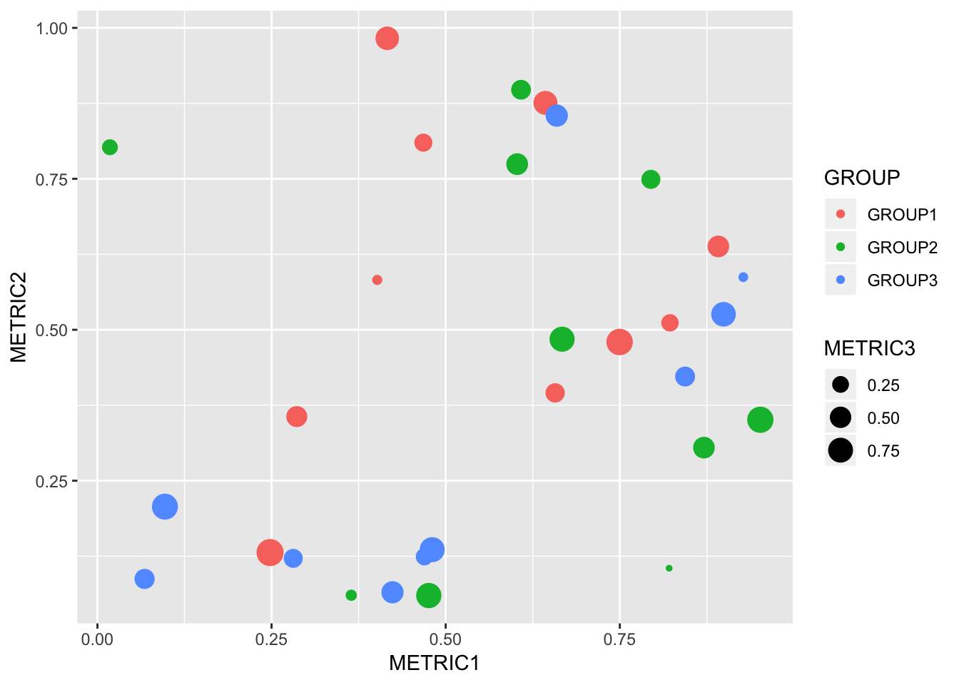
That’s all for now. Give me a shout if you have any questions or suggested improvements.
hasta luego!